


Abstract
In research on the determinants of change in health status, a crucial analytic decision is whether to adjust for baseline health status. In this paper, the authors examine the consequences of baseline adjustment, using for illustration the question of the effect of educational attainment on change in cognitive function in old age. With data from the US-based Assets and Health Dynamics Among the Oldest Old survey (n = 5,726; born before 1924), they show that adjustment for baseline cognitive test score substantially inflates regression coefficient estimates for the effect of schooling on change in cognitive test scores compared with models without baseline adjustment. To explain this finding, they consider various plausible assumptions about relations among variables. Each set of assumptions is represented by a causal diagram. The authors apply simple rules for assessing causal diagrams to demonstrate that, in many plausible situations, baseline adjustment induces a spurious statistical association between education and change in cognitive score. More generally, when exposures are associated with baseline health status, this bias can arise if change in health status preceded baseline assessment or if the dependent variable measurement is unreliable or unstable. In some cases, change-score analyses without baseline adjustment provide unbiased causal effect estimates when baseline-adjusted estimates are biased.
Epidemiologists frequently examine statistical relations between an exposure of interest (e.g., educational attainment) and a measure of change in health status (e.g., change in cognitive status). A key analytic decision is whether to condition on baseline health status, for example, by using regression adjustment, stratification, restriction, or matching. This paper examines the rationale for and consequences of adjusting for baseline values of the dependent variable in models of change. We catalogue a number of biases that can plague observational studies of change in health status. We argue that, although adjustment for baseline health status ameliorates certain biases, it introduces others and, in a typical study, the bias introduced by adjustment exceeds the bias eliminated. For clarity, we focus on a specific application: the putative effect of educational attainment on change in cognitive function in old age.
We present an empirical example using data from the US-based Assets and Health Dynamics Among the Oldest Old (AHEAD) study. Coefficient estimates for the effects of education on cognitive change increase substantially when baseline cognitive score is included as an independent variable in regression models, compared with models without baseline adjustment. Explaining this discrepancy was the motivation for this paper. We need a systematic method to determine which, if either, coefficient estimate is “right.” Directed acyclic graphs (DAGs)—in which we map out the assumed causal relations among the exposure, potential covariates, and outcome—provide such a method. DAGs can be used to determine whether the coefficient estimate from either analysis (with or without baseline adjustment) equals the causal effect of interest under a given set of assumptions. We represent plausible assumptions about relations among the variables of interest by using DAGs. The plausibility of assumptions partially depends on researchers' prior beliefs. To justify our assumptions, we draw on two well-accepted epidemiologic phenomena: regression to the mean and horse racing. We then apply simple rules for DAGs to demonstrate that, contrary to common intuition, baseline adjustment often fails to remove confounding and sometimes induces spurious correlation between exposure and measured health change. If baseline cognitive function and exposure are strongly associated, biases induced by baseline adjustment can be quite large. Baseline adjustment is occasionally advantageous, but whether it eliminates or introduces bias depends crucially upon the causal structure relating the variables.
Our arguments use DAGs instead of other approaches because DAGs are easily modified to accommodate alternative substantive assumptions and entail minimal mathematics (although the rules we apply to DAGs are mathematically grounded). The relations we demonstrate with DAGs could be, and in some cases already have been, proven mathematically (1, 2) or modeled with simulation studies.
We begin by specifying the causal question of interest and some background assumptions. Individuals begin life with different levels of cognitive ability, encounter exposures throughout life that alter that ability, and typically experience decline in some abilities during old age. Different individuals experience different rates of decline. We are interested in determining whether education, usually completed early in life, affects rates of cognitive decline in old age (temporal order as shown in figure 1). We adopt a counterfactual account of causation, contrasting the actual cognitive decline experienced by each individual, given his or her actual level of education, with the cognitive decline that person would have experienced had he or she received more or less education. If the amount of decline experienced given these two circumstances differs, then education affects cognitive decline. This issue is distinct from education's effect on elder cognitive impairment (i.e., function below a fixed threshold). In fact, if education affects cognitive function or reserve in middle age, then it will affect the incidence of cognitive impairment in later life, even if it has no effect on the rate of cognitive decline in old age (3).
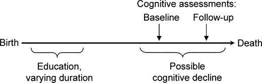
Assumed temporal order of education, cognitive change, and cognitive assessments among participants in the Assets and Health Dynamics Among the Oldest Old study born before 1924, United States.
MATERIALS AND METHODS
Sample data
AHEAD is a nationally representative cohort study of people born before 1924. Descriptions of this study, including measurement validation, are published elsewhere (4–7); appendix 1 provides further details. Interviews were conducted in 1993, 1995, 1998, and 2000. Our analyses include only those individuals who completed a baseline cognitive assessment (n = 5,726).
Cognitive assessment was based on the Telephone Interview for Cognitive Status, plus delayed recall of a 10-word list (possible range, 0–35) (8). Cognitive scores were considered missing if immediate recall, delayed recall, or four or more Telephone Interview for Cognitive Status items were missing. When fewer than four such items were missing, the score was calculated as the number of correct answers divided by the percentage of items completed.
We assume that these cognitive test scores reflect some random variation around true cognitive function due to measurement error or instability (transient fluctuations in cognitive function attributable to illness, for example) in function itself (6). Throughout this paper, we distinguish between cognitive function, a biologically based human capacity, and cognitive score, the measure of that capacity. Similarly, we distinguish between change in cognitive function and change in cognitive score. We assume that scientific interest is in change in function rather than the surrogate measure, change in cognitive score. Participants were aged 70 years or older at enrollment; they may have experienced both age- and education-related cognitive changes prior to baseline cognitive assessments.
Education (years of schooling completed) was reported in 1993. Variables that may affect both education and cognitive change were also included as regression covariates: age at interview, age squared, race (Black vs. all others), Hispanic ethnicity, and sex.
Statistical analyses
Our interest is in whether either education coefficient (γ1 or β1) provides an unbiased estimate of the effect of education on cognitive change. When parameter estimates from the two models differ, at least one estimate is incorrect with respect to the causal question we posed. Models were estimated with linear regression by using Stata 8.0 statistical software (Stata Corporation, College Station, Texas). To show the consistency of the findings, we repeated the analyses by using change in cognitive score over four time intervals: 1993–1995, 1995–1998, 1998–2000, and 1993–2000.
The AHEAD study used a complex sampling design that included cluster sampling (4). Therefore, we constructed confidence intervals by using the bootstrap with resampling (500 draws) of clusters (9).
Graphical models
Causal DAGs visually encode an investigator's a priori assumptions about causal relations among the exposure, outcomes, and covariates. The d-separation rules can be applied to identify the statistical relations implied by these causal assumptions (these rules, and an explanation of how to determine the statistical relations implied by a DAG, are summarized in appendix 2 and figure 2). To demonstrate biases potentially induced by baseline adjustment, we specify a number of alternative DAGs representing plausible relations among education, baseline cognitive function, baseline cognitive score, change in function, change score, and background variables. All DAGs impose the null hypothesis that education does not affect change in function either directly (indicated by the absence of an arrow from education to change in function) or indirectly via baseline function (indicated by the lack of an arrow from baseline function to change in function). We use the d-separation rules to determine whether, under the assumptions represented by each model, education and change score are statistically independent (unassociated) conditional on (adjusting for) baseline cognitive score.
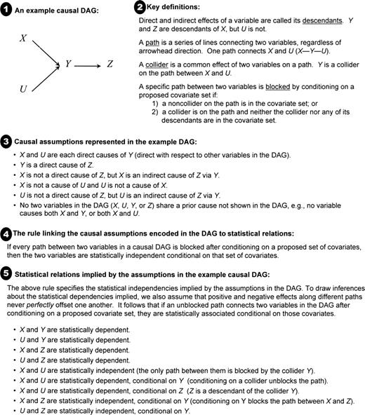
Introduction to directed acyclic graphs (DAGs), which visually represent assumptions about the causal relations among variables. Simple rules specify the statistical relations implied by these causal assumptions, assuming a large enough sample so that random variations can be ignored. Refer to appendix 2 and to Greenland et al. (40) (Epidemiology 1999;10:37–48) for a detailed discussion.
If education and change score are statistically associated after conditioning on baseline cognitive test score, under the null hypothesis, baseline-adjusted analyses are by definition biased regarding the (null) effect of education on change in function. For each DAG, we likewise consider whether an analysis without adjustment for baseline cognitive score is valid by determining whether education and change score are statistically independent without adjustment for baseline score (under the assumptions represented in the DAG). The null assumption of no causal effect on cognitive change is adopted for simplicity; the biases we discuss also apply under alternative hypotheses.
When discussing DAGs, we assume that positive and negative causal effects never perfectly offset one another (e.g., if education promotes cognition via one pathway but harms cognition via another pathway, we assume that the absolute magnitudes are not exactly identical, so education is either positively or negatively statistically associated with cognition). Our theoretical discussion supposes large samples so that effects due to random variation can be ignored.
RESULTS
Empirical findings
Descriptive characteristics of AHEAD study sample members, by educational level, are given in table 1. Substantial attrition occurred during follow-up. For simplicity, analyses are based on available cases; accounting for attrition with sophisticated methods would not affect the methodological issues we discuss. Table 2 shows mean cognitive scores and change scores, by level of education. At each wave, higher educational attainment predicted better cognitive scores but was unrelated to change scores.
Characteristics of Assets and Health Dynamics Among the Oldest Old study participants born before 1924, by level of education, United States*
<12 years of schooling | 12 years of schooling | >12 years of schooling | |||||||
|---|---|---|---|---|---|---|---|---|---|
| No. | % | No. | % | No. | % | ||||
| No. | 2,147 | 100 | 1,833 | 100 | 1,746 | 100 | |||
| Male | 855 | 40 | 627 | 34 | 751 | 43 | |||
| Black | 370 | 17 | 122 | 7 | 102 | 6 | |||
| Hispanic | 200 | 9 | 36 | 2 | 25 | 1 | |||
| Birth year | |||||||||
| <1910 | 359 | 17 | 169 | 9 | 249 | 14 | |||
| 1910–1914 | 528 | 25 | 346 | 19 | 335 | 19 | |||
| 1915–1919 | 663 | 31 | 615 | 34 | 534 | 31 | |||
| 1920–1923 | 597 | 28 | 703 | 38 | 628 | 36 | |||
| Not in sample in 2000 | 1,271 | 59 | 789 | 43 | 723 | 41 | |||
| Known to be deceased by 2000 | 788 | 37 | 521 | 28 | 483 | 28 | |||
Included are age-eligible enrollees for whom a valid 1993 cognitive assessment was available. Respondents may be both Black and Hispanic. Distributions are calculated without sampling weights; thus, the distributions are not representative of the national population.
No. | <12 years of schooling | 12 years of schooling | >12 years of schooling | |
|---|---|---|---|---|
| 1993 cognitive score | 5,726 | 17.8 (5.3) | 21.4 (4.6) | 22.4 (4.6) |
| 1995 cognitive score | 4,428 | 18.7 (5.0) | 21.7 (4.5) | 22.6 (4.5) |
| 1998 cognitive score | 3,633 | 18.3 (5.2) | 21.2 (4.7) | 22.3 (4.8) |
| 2000 cognitive score | 2,943 | 18.3 (4.9) | 20.8 (4.6) | 22.0 (4.6) |
| Change score 1993–1995 | 4,428 | −0.3 (4.2) | −0.4 (4.2) | −0.3 (4.2) |
| Change score 1995–1998 | 3,430 | −1.0 (4.0) | −0.8 (4.1) | −0.7 (4.0) |
| Change score 1998–2000 | 2,782 | −1.0 (4.0) | −1.0 (4.2) | −1.1 (4.0) |
| Change score 1993–2000 | 2,943 | −1.6 (4.7) | −1.8 (4.6) | −1.7 (4.6) |
Values are presented as mean (standard deviation).
Included are age-eligible enrollees for whom a valid 1993 cognitive assessment was available. Distributions were calculated without accounting for study design.
No. | <12 years of schooling | 12 years of schooling | >12 years of schooling | |
|---|---|---|---|---|
| 1993 cognitive score | 5,726 | 17.8 (5.3) | 21.4 (4.6) | 22.4 (4.6) |
| 1995 cognitive score | 4,428 | 18.7 (5.0) | 21.7 (4.5) | 22.6 (4.5) |
| 1998 cognitive score | 3,633 | 18.3 (5.2) | 21.2 (4.7) | 22.3 (4.8) |
| 2000 cognitive score | 2,943 | 18.3 (4.9) | 20.8 (4.6) | 22.0 (4.6) |
| Change score 1993–1995 | 4,428 | −0.3 (4.2) | −0.4 (4.2) | −0.3 (4.2) |
| Change score 1995–1998 | 3,430 | −1.0 (4.0) | −0.8 (4.1) | −0.7 (4.0) |
| Change score 1998–2000 | 2,782 | −1.0 (4.0) | −1.0 (4.2) | −1.1 (4.0) |
| Change score 1993–2000 | 2,943 | −1.6 (4.7) | −1.8 (4.6) | −1.7 (4.6) |
Values are presented as mean (standard deviation).
Included are age-eligible enrollees for whom a valid 1993 cognitive assessment was available. Distributions were calculated without accounting for study design.
Table 3 compares estimated regression coefficients for years of education from alternative models. The upper panel shows cross-sectional regression results; a single year's cognitive test score was used as the dependent variable. Education is significantly (p < 0.01) associated with cognitive scores in every year.
Regression coefficients for years of education in models of cognitive score and cognitive change score for Assets and Health Dynamics Among the Oldest Old study participants born before 1924, United States
β | 95% confidence interval | |
|---|---|---|
| Cross-sectional regressions | ||
| 1993 cognitive score | 0.55 | 0.52, 0.59 |
| 1995 cognitive score | 0.46 | 0.43, 0.49 |
| 1998 cognitive score | 0.49 | 0.45, 0.52 |
| 2000 cognitive score | 0.45 | 0.41, 0.49 |
| Change-score models without baseline adjustment | ||
| Change 1993–1995 | −0.02 | −0.05, 0.01 |
| Change 1995–1998 | 0.02 | −0.01, 0.06 |
| Change 1998–2000 | 0.00 | −0.04, 0.04 |
| Change 1993–2000 | −0.03 | −0.07, 0.01 |
| Change-score models with baseline adjustment | ||
| Change 1993–1995 | 0.20 | 0.17, 0.23 |
| Change 1995–1998 | 0.21 | 0.17, 0.23 |
| Change 1998–2000 | 0.19 | 0.16, 0.22 |
| Change 1993–2000 | 0.24 | 0.20, 0.27 |
The middle panel of table 3 shows education coefficients from change-score models without baseline adjustment. Education does not predict change in cognitive score in any of the four time intervals. The bottom panel shows change-score models with baseline adjustment. In every interval, higher education significantly predicts better change scores when conditioning on baseline cognitive score.
Are the coefficients credible?
Several empirical findings cast doubt on the causal validity of coefficient estimates derived from baseline-adjusted models. Baseline adjustment inflates the education coefficient relative to models without baseline adjustment, suggesting that baseline score is not a proxy for positive confounders of the relation between education and cognitive change. If education slows cognitive decline, the cross-sectional gradient in cognitive scores across educational levels should become increasingly steep at older ages as the longitudinal effects accumulate. This does not occur; the test-score advantage associated with education is stable over time. Similarly, if baseline-adjusted coefficients reflect causal relations, these coefficients would likely be larger for longer follow-up periods. Instead, the education coefficient for change from 1993 to 1995 is similar to the coefficient estimate for change from 1993 to 2000. We next explore causal mechanisms that could be responsible for the discrepancy between baseline-adjusted and -unadjusted results. Below, we describe some conditions under which unadjusted analyses are valid but the adjusted analyses would be biased under the null hypothesis.
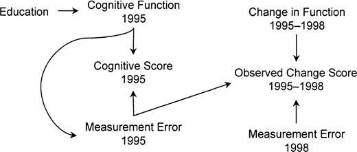
A DAG to demonstrate that regression to the mean may bias baseline-adjusted analyses
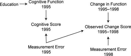
Directed acyclic graph assuming measurement error in baseline cognitive function for participants in the Assets and Health Dynamics Among the Oldest Old study born before 1924, United States. The absence of an arrow from education to change score shows the assumption that education does not affect decline due to aging (the null hypothesis). Education affects cognitive function, which in turn affects cognitive score. Cognitive score is an imperfect measure of cognitive function because of measurement error. This error directly affects the observed change score. Education is marginally uncorrelated with change score but is correlated when adjusted for 1995 cognitive score.
If we assume that figure 3 is correct, education and change score are statistically independent (uncorrelated) as desired under the null hypothesis. In DAG terminology, the only path in the diagram connecting education and change score (education–function1995–score1995–error1995–change score) is blocked by score1995 (a collider). Thus, analyses not adjusted for score1995 provide unbiased estimates of the overall (i.e., total) effect of education on change.
Conditional on score1995, however, education and change score are spuriously correlated, because conditioning on a collider “unblocks” the path. This phenomenon can be intuitively explained as follows. Anyone with a high score1995 has either a high function1995 or a large positive measurement error1995 (or both). A low-functioning person with a high score1995 must have a positive error1995; similarly, if a high-functioning person scored poorly, it was due to a negative error. Thus, within levels of score1995, function1995 and error1995 are inversely correlated and education and error1995 are inversely correlated. Because error1995 and error1998 are independent and error1995 contributes negatively to change score, change score and error1995 are negatively correlated: an example of the regression to the mean phenomenon. Hence, conditional on score1995, education and change score are positively correlated. Therefore, baseline-adjusted education coefficients are positive, even when education does not affect cognitive decline. The spurious correlation is proportional to the error in the cognitive measures and the strength of the education–function1995 relation (1). Instability has the same consequence as measurement error.
The education coefficient ψ1 in equation 5 is the direct effect of education on function1998 not mediated by function1995 and is also equal to the direct effect of education on change in function. Therefore ψ1 is zero because of the absence of an arrow from education to change in function (figure 3).
Model 6 is simply model 5, except that the independent variable function1995 is now measured with error. The education coefficient in equation 6 is identical to that in the baseline-adjusted change score model shown in equation 1 (11). The regression coefficient for an unreliably measured covariate, for example,
Is it possible that the DAG shown in figure 3 could have generated the AHEAD data and that the entire magnitude of the baseline-adjusted estimate is attributable to measurement error and regression to the mean? We show that the answer is yes. Specifically, if the baseline measure's reliability (the squared correlation between true function and test score) is known, structural equation modeling (12) or Yanez's bias formula (13) can be used to estimate the magnitude of bias attributable to measurement error and regression to the mean under the assumption that figure 3 generated the data and that linearity assumptions hold. By using cognitive test score reliability estimates of 0.8–0.6, as reported in the literature (7), we calculated that baseline adjustment induces a bias in the regression coefficient for education in the range of 0.10–0.21. This range includes our estimates of the education effect from the baseline-adjusted models fit to the AHEAD data. In fact, the actual bias could be even greater because the reported reliability estimates (7) did not account for transient fluctuations in cognitive function and thus may be too high.
By modifying the figure 3 DAG to represent different assumptions, we can examine whether baseline-adjusted models are biased under alternative scenarios. In each case below, provided that the other assumptions in figure 3 hold, adjustment for an imperfectly measured baseline score biases the estimated effect of education on cognitive change, while models without baseline adjustment are unbiased.
Function1995 and error1995 share a prior cause.
Function1995 directly affects change in function1995–1998.
Function1995 and education are correlated because of a common prior cause.
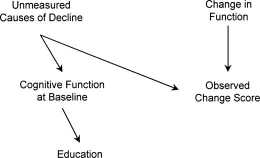
A DAG to demonstrate that horse racing may bias baseline-adjusted analyses
The DAG in figure 3 encodes the assumption that function1995 and change in function from 1995 to 1998 have no prior common causes. This assumption is unrealistic if factors besides education cause cognitive change prior to the baseline assessment in 1995. Factors that affected cognitive changes prior to baseline, for example, genetic background or lifestyle, may continue to operate during follow-up. The DAG in figure 4 represents the assumption that unmeasured factors besides education induced decline before the 1995 assessment and continue to cause cognitive changes from 1995 to 1998. For simplicity, this figure assumes that measurement error is absent. Under this causal model, education is marginally independent of change in cognitive score: all paths are blocked by colliders. Conditional on function1995, however, education and change score are correlated.
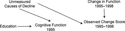
Directed acyclic graph showing the horse-racing effect for participants in the Assets and Health Dynamics Among the Oldest Old study born before 1924, United States. If decline began prior to 1995, baseline cognitive function will reflect that decline. Under the assumptions in this graph, education is marginally uncorrelated with change score but is correlated when adjusted for 1995 cognitive function.
This is in contrast to typical omitted variable bias, in which bias occurs because we fail to adjust for common causes of the exposure and the outcome. This phenomenon is instead related to what Peto dubbed the horse-racing effect: “[I]n a race between fast and slow horses … one would expect to find the faster horses out in front halfway through the race” (14, p. 467). Assessing baseline cognitive status after decline has already begun is analogous to peeking at the order of the horses halfway through a race: if decline began before 1995, function1995 tends to be worse for individuals who are fast decliners. Function1995 is thus influenced by both education and other causes of decline. Conditioning on function1995 creates a spurious correlation between its causes (education and unmeasured causes of decline). The spurious correlation between education and other causes of decline induces a spurious relation between education and change score within levels of function1995.
Unlike the bias induced by regression to the mean discussed previously, this bias occurs even if baseline cognitive function is measured without error. Quantifying horse-racing bias requires additional assumptions. In the simplest case—no interaction between education and unmeasured causes of decline—it biases effect estimates downward.
Using the DAGs to interpret AHEAD results
Either substantial measurement error or horse racing, or both, will almost always be present; thus, in practice, the bias introduced by baseline adjustment can be large. As a result, baseline adjustment will generally result in sizable bias. In particular, we think that this is the case with the AHEAD data.
We therefore conclude that these analyses of the AHEAD data provide no evidence that education beneficially influences cognitive change in old age. This finding does not conclusively demonstrate that education has no benefit for cognitive change, because, under plausible causal structures, both baseline-adjusted and -unadjusted models are biased even when no unmeasured common causes of education and cognitive change exist.
One such setting occurs when cognitive tests have ceilings (or floors). Everyone whose function exceeds the ceiling is assigned the same, maximum, score. Thus, cognitive function influences measurement error (figure 5): the greater the cognitive function, the more negative the error. In this DAG, an unblocked path connects education and change score. Conditioning on function1995 would block this path, but conditioning on score1995 does not. Therefore, in contrast with the DAGs shown in figures 3 and 4, analyses both with and without baseline adjustment are biased for the (null) effect of education on change in function. Under additional assumptions, nonstandard analyses based on Tobit or censored median regression models, without baseline adjustment, can be used to ameliorate ceiling and floor problems (15–19). In these models, scores that equal the ceiling values are regarded as censored. Unfortunately, as we show in appendix 3, not even censored regression methods solve other scaling problems, such as noninterval scales (20, 21).
Directed acyclic graph showing the effect if measurement error differs by baseline cognitive function for participants in the Assets and Health Dynamics Among the Oldest Old study born before 1924, United States. Measurement error may depend in part on cognitive function, for example, because of a ceiling on the scale. In this graph, education will potentially be correlated with change score in a model adjusted for 1995 cognitive score or a model without such adjustment. Both the baseline-adjusted and -unadjusted models will show a correlation, which is spurious under the null hypothesis.
DISCUSSION
The baseline adjustment problem, sometimes discussed in the context of Lord's Paradox (22), covariance adjustment, or gain scores (23), has generated an extensive literature (1, 24–27). We argue that substantive arguments sometimes used to defend baseline adjustment are largely misleading.
Misperceptions about the advantages of baseline adjustment
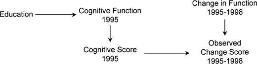
Common justifications for baseline adjustment are that it improves efficiency, eliminates confounding, or avoids bias due to measurement ceilings or floors. Concerns about efficiency are generally secondary to concerns about bias and consistency, so we focus on examples in which baseline-adjusted change-score models provide unbiased effect estimates.
Consider figure 6, in which, unlike the AHEAD study, baseline function is a cause of exposure and baseline adjustment eliminates confounding. Education and change score share a prior cause (unmeasured causes of decline), so the marginal statistical relation between these two variables does not reflect the causal relation. However, adjusting for baseline cognitive function controls confounding, provided that we have an error-free baseline measure. Note that if unmeasured common causes positively affect both education and cognitive change, then baseline adjustment would reduce the coefficients relative to coefficients from unadjusted models.
Directed acyclic graph showing the effect when assuming a common prior cause of education and cognitive change and no measurement error for participants in the Assets and Health Dynamics Among the Oldest Old study born before 1924, United States. If baseline cognitive function affects education, and decline has begun by the time the baseline assessment is conducted, adjusting for baseline function will not induce a correlation between education and observed change score.
Even in studies in which baseline function is measured prior to exposure and is an important confounder, adjustment for baseline score introduces regression-to-the-mean bias if baseline function is measured with error. In this setting, structural equation modeling (12) or Yanez's bias formula (13) can sometimes be used to control confounding by baseline function while avoiding regression-to-the-mean bias. In other cases, it is impossible to obtain unbiased effect estimates. By using prior evidence regarding the direction or magnitudes of the causal relations, however, it may be possible to determine the direction of bias and thus establish a plausible range for the true causal effect.
Furthermore, baseline adjustment does not eliminate common scaling problems associated with cognitive outcomes, such as ceilings or floors, except under special circumstances (detailed in appendix 3) that would rarely, if ever, apply. Scaling problems are crucial; as shown in appendix 3, education may affect change score on one scale but not on another. In summary, baseline-score adjustment eliminates all confounding under special circumstances only, and it often induces bias. Situations in which baseline adjustment provides unbiased estimates can be identified by specifying the assumed causal relations among the variables.
Analyses that implicitly condition on baseline
Adjustment in regression models is only one form of conditioning on baseline score. Stratifying or matching on baseline score, excluding high- or low-scoring individuals from analyses, and normal score transformation of change scores within level of baseline score can all induce similar biases. These remarks apply to logistic regression or proportional hazards regression as well as to linear regression.
Baseline-adjusted analyses in prior literature on education and cognitive change
A recent review identified 14 longitudinal studies of education and cognitive change, 12 of which found some benefit of education (28). Of the 12 positive studies, eight explicitly conditioned on baseline performance (29–36). This review suggests that the jury is still out regarding the relation between education and cognitive change: the majority of studies addressing the research question have a potentially serious methodological problem that could entirely account for their findings. For example, reanalysis of the data reversed the positive results from one of the baseline-adjusted studies reviewed above (34). The later analysis incorporated a third assessment wave and used latent growth curve modeling without baseline adjustment. No relation between education and rate of change in cognitive function was observed (37).
Other methodological problems, for example, noninterval scales, competing risks, or differential attrition, are common in studies of education and cognitive change, including our analysis. These issues must also be resolved to allow a confident conclusion about the effect of education on cognitive change.
Conclusion
We have shown that baseline adjustment substantially alters coefficient estimates in analyses of the effect of education on cognitive change. Any of several causal structures could account for a discrepancy between baseline-adjusted and baseline-unadjusted models. In general, if exposure predicts baseline level of the outcome, conditioning on this baseline measure induces a spurious correlation between the exposure and change score in either of two common situations:
Measures of the outcome fluctuate because of imperfect measurement reliability or latent variable instability; or
Change has already occurred prior to the baseline measurement, the rate of change experienced in the past predicts the future rate of change, and exposure is unaffected by baseline function.
Whenever either of these criteria is met, exposure is likely to be a statistically significant predictor in baseline-adjusted change-score regression models even under the null assumption of no causal effect of exposure on change. Similarly, if there is a causal effect, baseline-adjusted models generally provide biased effect estimates. In many cases, models without baseline adjustment are unbiased, but, under some causal structures, an unbiased effect estimate cannot be derived with either baseline-adjusted or -unadjusted models. Such situations are easily assessed with DAGs, allowing analysts to seek alternative, unbiased methods or, at a minimum, attempt to quantify the magnitude of alternative biases.
We have focused on cognition, but the problems apply to many other outcomes. When prior assumptions about the underlying relations are clearly specified in causal diagrams, simple rules can be used to determine whether proposed analyses consistently estimate the causal effect of interest. It may be impossible to derive unbiased estimates of the effect of education on cognitive change by using standard analyses of the data typically available in large surveys. These problems are not insurmountable, however. We can make progress on this research question by providing evidence on the measurement properties of cognitive instruments, explicitly modeling latent variables, pursuing censored data approaches, and eliminating competing causal models by ruling out (or in) possible confounders.
APPENDIX 1
Details on the AHEAD Data Set
AHEAD is a nationally representative sample of community-based individuals born before 1924. Respondents were selected by using a dual-frame multistage probability sample. The primary sampling stage used US Metropolitan Statistical Areas and non–Metropolitan Statistical Area counties. In the 66 primary sampling units selected, secondary sampling unit areas were selected, and houses were enumerated. The third sampling stage involves systematic selection of housing units within the secondary sampling unit. The design oversampled African Americans, Mexican Hispanics, and residents of the state of Florida by increasing the probability of selecting sampling areas with a high proportion of African Americans or Mexican Hispanics. For respondents born before 1914, a second sampling frame was used. This list was drawn from the Health Care Financing Administration's listing of Medicare enrollees in selected counties. Both sampling frames excluded elderly living in institutions.
The baseline AHEAD interviews occurred in 1993. The survey covered three major domains—health, financial circumstances, and family—in as much detail as possible within the goal of a 1-hour interview. Our analyses made little use of the detailed information about the adult life of AHEAD respondents because education is believed to temporally precede and most likely affect the majority of these characteristics. Thus, we selected covariates that preceded education. Surviving respondents were recontacted in 1995, 1998, and 2000; the survey is ongoing.
APPENDIX 2
Introduction to using DAGs
In DAGs, arrows between variables represent the investigator's a priori assumptions about the causal relations among the potential covariates, the exposure, and the outcome. When these assumptions are represented in a DAG, a simple rule (described below) can be applied to select a set of covariates to include in a regression model. We seek a set of covariates such that, after adjusting for these covariates, the statistical association between the exposure and the outcome of interest equals the causal effect of the exposure on the outcome. For example, if the exposure does not affect the outcome, then we want a covariate set such that, after adjusting for these covariates, the correlation between the exposure and the outcome is zero.
Formal introductions to graphical models and proof of the mathematical equivalence between the rules we apply to DAGs and Robins's g-computation formula can be found elsewhere (38–42). Here, we informally introduce the rules for identifying the conditional independencies implied by a DAG, that is, determining whether the causal assumptions represented in the DAG necessarily imply that two variables are statistically independent conditional on a proposed covariate set. To relate this discussion to more common epidemiology terms, note that regression coefficients, t statistics, odds ratios, and the like are examples of measures of statistical dependence between variables. Covariate adjustment in a regression model is a type of conditioning, as are stratification and matching.
Formally, the rules we apply to DAGs state the statistical independencies implied by the assumptions in the DAG. For this paper, we assume that positive and negative causal effects never perfectly offset one another. This additional assumption extends the rules to specify the statistical dependencies implied by the DAG, as discussed later. To make this introduction less technical, we also assume a large sample so that effects due to random variation can be ignored.
In a causal DAG, we say that a variable X causes a variable Y directly (relative to the other variables in the DAG) if there is an arrow from X to Y or indirectly if there is a sequence of directed arrows that can be followed from X to Y via one or more intermediate variables. In figure 2, X causes Y directly and Z indirectly. Direct and indirect effects of a variable are called descendants of that variable. If two variables shown in a DAG share a common cause, that common cause must also be included in the DAG. It is not necessary to include all causes of individual variables in the model; only causes of two or more variables in the DAG must be included. If unknown or unmeasured common causes are assumed to exist, they should be represented in the diagram as unknown common causes with arrows to the variables they are thought to affect. The absence of a sequence of directed arrows linking two variables in a DAG represents the assumption that there is no causal relation between the two variables. If a prior value of Y affects X, which affects a subsequent value of Y, these must each be shown as separate variables (e.g., Y0→X1→Y2). DAGs do not have any cycles between variables, consistent with the general intuition that if X causes Y, Y cannot also cause X at the same moment.
The DAG expresses a set of assumptions about the causal relations or absence of causal relations among the variables. If the assumptions of a causal DAG are correct, then two variables in the DAG will be statistically independent conditional on a set of covariates if every “path” between the two variables is “blocked.” Likewise, they will be statistically dependent if there is an unblocked path between them, setting aside the unlikely possibility of perfectly counterbalancing paths. What is a path, and what does it mean to block it? A path is any sequence of lines (also called edges) connecting two variables regardless of the direction of the arrowheads. The direction of arrowheads is important to identify variables on a path that are “colliders.” If arrowheads from A and B both point to a variable C (as in A→C←B), then C is referred to as a collider on that path between A and B: the causes collide at C. In other words, a collider is a common effect of two variables on the path (the collider itself must also be on the path). All other variables on a path are noncolliders. A path is blocked by a proposed set of variables if either of two conditions holds:
One of the noncolliders on the path is in the proposed covariate set; or
There is a collider on the path and neither the collider nor any of the collider's descendants is in the proposed covariate set.
These rules fit with the intuition that two variables will be correlated if there is a causal relation between them or if there is an uncontrolled prior common cause of the two variables. The rules also reflect the fact that a statistical association between two variables can be induced by conditioning on a common effect of the two variables (40, 43). Note that if a collider on a path is in the proposed covariate set, this collider does not block the path. If a DAG contains no unblocked paths between A and B, the two variables will be marginally independent; that is, without conditioning on any other variables, A and B will be independent. Rule 2 implies that conditioning on a variable may unblock a path between A and B and induce a correlation, if the variable is a collider or a descendant of a collider. The assumptions in the sample DAG in figure 2 imply that X and U are marginally independent but become statistically associated after conditioning on either Y or Z. In contrast, X and Z are marginally dependent but become statistically independent after conditioning on Y.
The assumption that positive and negative effects never perfectly offset one another is needed because two variables might be causally connected but nonetheless statistically independent if connected by two perfectly counterbalanced pathways. If perfectly counterbalanced pathways are possible, causal connections do not necessarily imply statistical dependencies. In the context of this paper, this assumption is mostly important when we discuss parameter estimates with multiple—possibly competing—sources of bias. If two sources of bias perfectly offset one another, the parameter estimate might be correct. We ignore this possibility and assume that parameter estimates with multiple sources of bias are themselves biased.
APPENDIX 3
Conditions under which an Adjusted Analysis Is Valid
Directed acyclic graph showing what occurs if baseline score is a perfectly measured, nonlinear transformation of function for participants in the Assets and Health Dynamics Among the Oldest Old study born before 1924, United States. In this graph, 1995 cognitive function is the only determinant of 1995 cognitive score, but this relation is nonlinear so that baseline score affects change score, although it is independent of change in function. Conditioning on baseline function or score will give an unbiased effect estimate for education, but analyses without baseline adjustment will be biased.
In appendix figure 1, although change1995–1998 is not affected by education, change score is causally affected by education. Furthermore, education and change score are independent conditional on score1995 but are unconditionally associated. The unconditional association between education and change score is an unbiased estimate of the effect of education on change score but a biased estimate of the effect of education on change in function. Thus, in this example, the unadjusted analysis is biased and baseline adjustment eliminates the bias.
If the function g is linear and deterministically maps both function1998 onto score1998 and function1995 onto score1995, then, on the DAG shown in appendix figure 1, the arrow from score1995 to change score is no longer present. As a consequence, there will be no unconditional association between education and change score. Under these assumptions, analyses that do not adjust for baseline will be unbiased, as will analyses that do adjust for baseline.
When g is nonlinear, change score can be viewed as change in function, except that it is measured on a different scale. Because education affects baseline cognitive function, it is possible for education to simultaneously have no effect on change in function and yet have a non-null effect on change in some nonlinear transformation of function. For example, if the transformation g is the logarithm, education could simultaneously have no effect on change in function and yet have a non-null effect on change in log function. That is, education may not affect change in function on an additive scale and yet still have an effect on a relative scale that measures fractional or percent change in function. Such “across-scale inconsistency” can occur only when education has a causal effect on baseline function1995. These previous statements refer to the overall (i.e., total) effect of education on change score. Across-scale inconsistency cannot exist for the direct effect of education on cognitive change (not mediated by baseline function), as is evident from appendix figure 1.
In summary, the DAG in appendix figure 1 characterizes a setting in which the direct effect of education on change score (not through score1995) can be validly estimated by an analysis that adjusts for baseline score, which is not the case if 1) an unmeasured common cause of function1995 and change in function (horse-racing effect) were added to the graph in appendix figure 1, or 2) if the ranking of some individuals on function1995 differed from their ranking on score1995. Condition 2 would apply if either score1995 has any (unmeasured) causes U besides function1995 or the reliability of the test measuring 1995 cognitive score was imperfect. These possibilities would be represented on appendix figure 1 by adding to the figure a variable U and/or a variable “measurement error in score1995” equal to {score1995 − g(function1995)} with arrows into score1995 and change score. Note that unless the transformation g is the identity transformation, this variable differs from the variable “measurement error 1995” shown in figures 3 and 6, which equals score1995 − function1995. Under condition 1 or 2, education and change score would be associated conditionally on score1995 even under the null hypothesis of no direct effect of education on change in function. As a consequence, the baseline-adjusted analyses would be biased. Either or both conditions 1 and 2 will almost always be present in practice. As a result, baseline adjustment will generally result in substantial bias.
In contrast, even if conditions 1 and 2 are present, an analysis unadjusted for baseline will, in the absence of additional unmeasured confounders, yield a valid estimate of the overall effect of education on change score. The remaining issue then becomes whether the score measured by the test battery is close to being a linear transformation of cognitive function. Because cognitive function has no agreed-upon operational definition, this latter question seems difficult to answer affirmatively without additional assumptions. In certain settings, such as when cognitive tests have ceilings (or floors), the answer is clearly in the negative.
This work was supported by grants from the National Institute of Aging (AG000158 and AG023399).
The authors gratefully acknowledge contributions from Drs. James Ware and Miguel Hernán in developing the ideas presented in this paper.
Conflict of interest: none declared.
References
Yanez ND, Kronmal RA, Shemanski LR. The effects of measurement error in response variables and tests of association of explanatory variables in change models.
Carroll RJ, Gallo P, Gleser LJ. Comparison of least squares and errors-in-variables regression, with special reference to randomized analysis of covariance.
Satz P. Brain reserve capacity on symptom onset after brain injury: a formulation and review of evidence for threshold theory.
Heeringa SG. Technical description of the Asset and Health Dynamics (AHEAD) survey sample design. Ann Arbor, MI: Institute for Social Research, University of Michigan,
Soldo B, Hurd M, Rodgers W, et al. Asset and Health Dynamics Among the Oldest Old: an overview of the AHEAD study.
Herzog AR, Wallace RB. Measures of cognitive functioning in the AHEAD study.
Ofstedal MB, McAuley GF, Herzog AR. Documentation of cognitive functioning measures in the health and retirement study. Ann Arbor, MI: Survey Research Center, University of Michigan,
Brandt J, Spencer M, Folstein M. The Telephone Interview for Cognitive Status.
Rust K, Rao J. Variance estimation for complex surveys using replication techniques.
Laird N. Further comparative analyses of pretest-posttest research designs.
Yanez ND, Kronmal RA, Shemanski LR, et al. A regression model for longitudinal change in the presence of measurement error.
Newey WK. Conditional moment restrictions in censored and truncated regression models.
Powell JL. Least absolute deviations estimation for the censored regression-model.
Jolliffe D, Krushelnytskyy B, Semykina A. Censored least absolute deviations estimator: CLAD. College Station, TX: Stata Press,
Stata 8 cross-sectional time-series reference manual, release 8. College Station, Texas: Stata Press,
Mungas D, Reed BR. Application of item response theory for development of a global functioning measure of dementia with linear measurement properties.
Alder AG, Adam J, Arenberg D. Individual-differences assessment of the relationship between change in and initial level of adult cognitive-functioning.
Allison PD. Change scores as dependent variables in regression analysis.
Rogosa D, Brandt D, Zimowski M. A growth curve approach to the measurement of change.
Anstey K, Christensen H. Education, activity, health, blood pressure and apolipoprotein E as predictors of cognitive change in old age: a review.
Shichita K, Hatano S, Ohashi Y, et al. Memory changes in the Benton Visual Retention Test between ages 70 and 75.
Evans DA, Beckett LA, Albert MS, et al. Level of education and change in cognitive function in a community population of older persons.
Farmer ME, Kittner SJ, Rae DS, et al. Education and change in cognitive function. The Epidemiologic Catchment Area Study.
Butler SM, Ashford JW, Snowdon DA. Age, education, and changes in the Mini-Mental State Exam scores of older women: findings from the Nun Study.
Christensen H, Korten AE, Jorm AF, et al. Education and decline in cognitive performance: compensatory but not protective.
Albert MS, Jones K, Savage CR, et al. Predictors of cognitive change in older persons: MacArthur studies of successful aging.
Arbuckle TY, Maag U, Pushkar D, et al. Individual differences in trajectory of intellectual development over 45 years of adulthood.
Christensen H, Hofer SM, Mackinnon AJ, et al. Age is no kinder to the better educated: absence of an association investigated using latent growth techniques in a community sample.
Spirtes P, Glymour C, Scheines R. Causation, prediction, and search. Cambridge, MA: MIT Press,
Greenland S, Pearl J, Robins JM. Causal diagrams for epidemiologic research.
Robins J. A graphical approach to the identification and estimation of causal parameters in mortality studies with sustained exposure periods.
Robins JM. Comment on Judea Pearl's paper, “Causal diagrams for empirical research.”

